
The NAOF's fiscal policy monitoring team has brought a regularly updated business cycle heatmap to the NAOF's website. The heatmap gives a real-time picture of the Finnish business cycle. The NAOF utilizes the heatmap in its fiscal policy analyses. You too can now utilize it to get a picture of the business cycle!
When fiscal policy is planned, implemented, and assessed, it is important to have available a reliable assessment of the prevailing phase of the business cycle. Therefore, the phase of the business cycle should be assessed using several different methods. One of the methods that the NAOF’s fiscal policy monitoring team has used in its analyses for a few years is the heatmap. In its previous reports, the team has utilized a heatmap based on quarterly observations. Further development has resulted in a more detailed heatmap that is more sensitive to cyclical fluctuations and based on monthly observations. This heatmap has now been published on the NAOF’s website to make it publicly available.
The heatmap makes it possible to assess the phase of the business cycle in Finland almost in real time. The heatmap is based on a model prepared by the Estonian Fiscal Council, and it has been adapted to the circumstances in Finland.
The heatmap consists of economic indicators
The heatmap examines the business cycle by monitoring the development of indicators illustrating the state of the Finnish economy. The indicators have been selected on the basis that historically, they have illustrated cyclical fluctuations accurately, monthly data is available on them, and they are linked to the development of GDP.
The heatmap uses statistics on the following eleven indicators: capacity utilization rate, unemployment rate, employment rate, vacancies, wages and salaries, consumer price index, and the sub-indicators of the Economic Sentiment Indicator (ESI): the industrial, services, consumer, construction, and retail trade confidence indicator. If necessary, indicators may be added, reduced, or exchanged. For the purposes of the heatmap, the indicator values are standardized to make them commensurate.
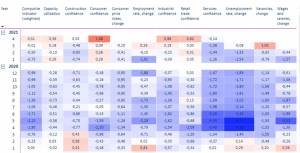
The colour of the heatmap changes according to the change in the indicator values. The red colour represents a situation where, based on the indicator in question, the economic activities exceed the average level, e.g. the employment rate improves, and salaries rise. Accordingly, blue represents a slowdown in economic growth. The higher the share of simultaneous red or blue indicators, the more likely the economy is to be experiencing good or bad times.
A monthly and annual composite indicator has also been compiled of the heatmap indicators
A composite indicator whose value is calculated from the heatmap variables has also been compiled of the individual cyclical indicators. The variables of the composite indicator have been weighted as follows: the weight of the sub-indicators of the Economic Sentiment Indicator (ESI) is 40% and that of each of the remaining variables is 10%. Thus, half of the weight is derived from real economic variables and half from sentiment indicators. The weights of individual variables of the ESI’s sub-indicators are updated in relation to each other according to the relative weights used by the Commission. The accurate weights are indicated in the table of variables on this page.
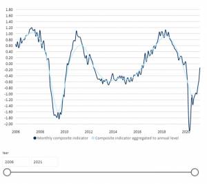
The figure shows the composite indicator values per month and per year. As shown in the figure, the monthly composite indicator illustrates the business cycle movement much more sensitively than the annual indicator. This is particularly evident in the observations of 2020 and the accuracy with which the indicator reacted to the Covid-19 crisis. As is clear from the figure, the monthly indicator was very sensitive to the sudden economic stop in Finland in April 2020.
The composite indicator and the output gap show a similar development
In Figure 3, the time series of the composite indicator is compared with the output gap for spring 2020, autumn 2020 and autumn 2019 calculated by the NAOF according to the method of the European Commission. In the long term, the output gap and the composite indicator have developed similarly, i.e. both methods provide a similar picture of the economic cycle and its phase and turning points, in particular.
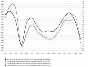
The output gap cannot be observed but is an estimate calculated by the NAOF using a production function method jointly agreed by the European Commission and its Member States. The method is applied to estimate the potential output in order to determine the output gap. The output gap is the difference between potential output and the output at a given time, i.e. GDP. The output gap gives the economic cycle a numerical value to be used in the calculation of the structural balance, i.e. in the calculation of the government deficit excluding cyclical fluctuations and one-off factors. The cyclical adjustment of the structural balance is carried out by means of an output gap estimated using a method jointly agreed by the EU Member States. The heatmap does not replace the output gap produced in this manner but can be used as reference data.
The composite indicator is revised over time only to a very small degree
The difference and benefit of the heatmap and the composite indicator based on it over the output gap is that the heatmap is based solely on such statistical data that are usually updated only to a small degree. In the case of the output gap, in turn, the picture of the economic situation may change significantly as the statistical data and forecasts used are updated.
Finland’s public debt ratio, i.e. the general government debt-to-GDP ratio, is currently high. The aim is to stabilize the debt ratio during this decade. The stabilization of the debt ratio is likely to require surpluses in public finances during an economic upturn, which failed in 2017–2019. After the Covid-19 pandemic, it is necessary to succeed in this. The possibility of success is enhanced by a clearer understanding of the current phase of the business cycle.